In a previous post I reviewed the basics of using the PerformanceAnalytics package in R for evaluating a simple 60/40 US stock/bond portfolio based on a pair of ETFs. Let’s round out that preliminary review by exploring a few additional applications before moving on to a deeper level of analysis in a future article, when we’ll consider the possibilities for enhancing a 60/40 mix.

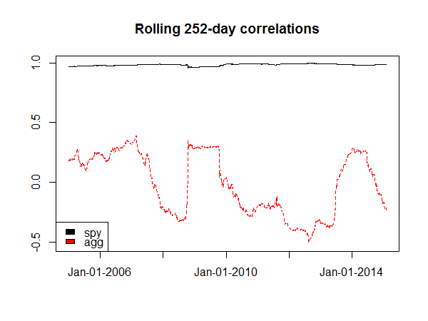
Meantime, the following code assumes that we’ve already loaded the data and relevant packages as discussed previously (see link above). Picking up where we left off, it’s often valuable to review correlation data for the individual assets relative to the portfolio. As an example, let’s create rolling correlations for trailing one-year windows. As you can see in the chart below, the equity component (SPY) tends to be highly correlated with the 60/40 portfolio while the bond allocation (AGG) exhibits low/negative correlation. No surprises here, although the chart summarizes the basic rationale for a stock/bond mix: diversification. (Note: plotting below is quite simple, and intentionally so. Creating publication-worthy plots in R is a detailed subject and so in the interest of code brevity I’ll stick with a basic charting application for now.)

[code language=”r”]
# create rolling correlations for 1yr windows (252 trading days) vs. rebalanced portfolio
spy.port.corr <-na.omit(runCor(x=portfolio.returns$spy,y=portfolio.rebal$returns,n=252))
agg.port.corr <-na.omit(runCor(x=portfolio.returns$agg,y=portfolio.rebal$returns,n=252))

# combine and label correlation data
spy.agg.port.corr <-cbind(spy.port.corr,agg.port.corr)
colnames(spy.agg.port.corr) <-c("spy","agg")

# create date file for plot
dates <-index(spy.agg.port.corr)

# plot correlation data
matplot(dates,spy.agg.port.corr,type="l",
xaxt="n",xlab="",
ylab="",
main="Rolling 252-day correlations")
axis.Date(side = 1, dates,format = "%b-%d-%Y")
legend("bottomleft",c(colnames(spy.agg.port.corr)),fill=palette())

[/code]

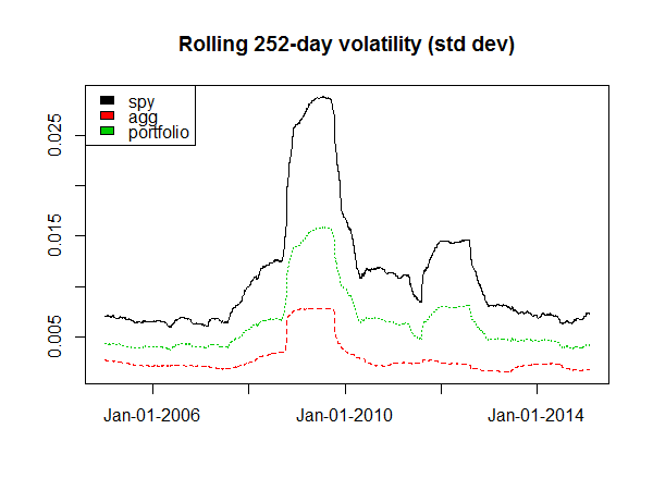
Next, let’s turn to volatility (standard deviation of daily returns). As you can see in the next chart, the rolling 252-day trading day vol numbers surged during the 2008 financial crisis. Not surprisingly, equity vol (black line) is highest and bond vol (red line) is relatively calm, with the overall portfolio (green line) of the two assets in the middle. The message, of course, is that owning a mix of stocks and bonds tames the volatility without (hopefully) giving up too much upside that’s associated (usually) with stocks.

[code language=”r”]

# create volatilty data
spy.port.vol <-na.omit(runSD(x=portfolio.returns$spy,n=252))
agg.port.vol <-na.omit(runSD(x=portfolio.returns$agg,n=252))
port.vol <-na.omit(runSD(x=portfolio.rebal$returns,n=252))

# combine and label volatility data
spy.agg.port.vol <-cbind(spy.port.vol,agg.port.vol,port.vol)
colnames(spy.agg.port.vol) <-c("spy","agg","portfolio")

# create dates file for plot
dates <-index(spy.agg.port.vol)

# plot correlation data
matplot(dates,spy.agg.port.vol,type="l",
xaxt="n",xlab="",
ylab="",
main="Rolling 252-day volatility (std dev)")
axis.Date(side = 1, dates,format = "%b-%d-%Y")
legend("topleft",c(colnames(spy.agg.port.vol)),fill=palette())

[/code]

Another valuable feature in the PerformanceAnalytics package is the ability to extract the fluctuating weights of the portfolio assets for analysis and monitoring purposes, perhaps with an eye on generating a rebalancing signal when one or more of the assets move beyond a specific threshold.

[code language=”r”]
# Review the weights for each asset
tail(portfolio.rebal$EOP.Weight)
spy agg
2015-01-26 0.5965518 0.4034482
2015-01-27 0.5934818 0.4065182
2015-01-28 0.5893674 0.4106326
2015-01-29 0.5917868 0.4082132
2015-01-30 0.5878612 0.4121388
2015-02-02 0.5908399 0.4091601

[/code]

We can also tap into the weighted return contribution for each asset. This is useful for identifying the main sources of a portfolio’s returns, for good or ill, over a given period. There’s not a lot of mystery on this front in a simple two-fund portfolio, but this feature comes in handy for portfolios with a wider spectrum of assets. In those cases, the main return drivers may not be obvious—unless we’re effectively x-raying the strategy by profiling return contributions. In the example below, all of the return contribution for 2015-02-02 for the portfolio was due to SPY; by contrast, AGG’s contribution for that day was nil.

[code language=”r”]
# Review the weighted return contribution for each asset
tail(portfolio.rebal$contribution)
spy agg
2015-01-26 0.001395437 -0.0001811544
2015-01-27 -0.007868851 -0.0002171216
2015-01-28 -0.007610993 0.0016781689
2015-01-29 0.005447835 -0.0003302970
2015-01-30 -0.007441648 0.0014605124
2015-02-02 0.007280106 0.0000000000
[/code]

Speaking of performance, generating the portfolio’s return history is straightforward…

[code language=”r”]
# Review portfolio returns, the sum of weighted returns for the assets
tail(portfolio.rebal$returns)
portfolio.returns
2015-01-26 0.001214283
2015-01-27 -0.008085972
2015-01-28 -0.005932824
2015-01-29 0.005117538
2015-01-30 -0.005981135
2015-02-02 0.007280106
[/code]

To verify that we’re looking at the portfolio’s performance, let’s manually run a check by summing the daily contributions via the apply() function…

[code language=”r”]
# verify portfolio returns by summing weighted returns for the assets
tail(as.xts(apply(portfolio.rebal$contribution,1,sum)))
[,1]
2015-01-26 0.001214283
2015-01-27 -0.008085972
2015-01-28 -0.005932824
2015-01-29 0.005117538
2015-01-30 -0.005981135
2015-02-02 0.007280106
[/code]

In an upcoming post I’ll consider some options for enhancing the risk-adjusted results of a standard 60/40 mix.