Deaccumulation is the new new thing in finance for an obvious reason: the US population is aging, which means that retirement becomes an increasingly pressing issue for financial planning. Perhaps the leading challenge for this critical task (other than accumulating a sufficient pot of money) is managing the withdrawals from a retirement portfolio. The task is a delicate balancing act of maximizing deaccumlation in the short term (over a one-year period, for instance) without running out of money before a retiree shuffles off this mortal coil. An absolute solution will always remain elusive due to the standard issues that bedevil finance, but some basic modeling applications can wrestle the uncertainty down to a comparatively tame beast.

Researchers have developed several techniques for modeling this problem, but in this post I’ll focus on the procedure outlined by M. Barton Waring and Laurence B. Siegel in an article published earlier this year in the Financial Analysts Journal (“The Only Spending Rule Article You Will Ever Need”, Jan/Feb 2015). The simplicity and economic logic of their work makes this a compelling starting point for bringing a degree of clarity to this critical financial-planning topic. In the analysis that follows, I’ll use R to crunch the numbers (the code is posted below), although you can also use Excel, as the authors do.

The main point of the article is to review the concept of “periodic re-annuitization.” Waring and Siegel explain that

We call a portfolio managed according to this principle an annually recalculated virtual annuity (ARVA)—“virtual” because the investor does not have to buy an actual annuity to reap many of the benefits of annuity thinking, even if she continues to hold a portfolio of risky assets.

Let’s make a few simplifying assumptions for illustrative purposes. First, we’ll model the future based on a 65-year-old investor with a $1 million portfolio for a 30-year time horizon. The goal in this academic exercise is to estimate optimal withdrawal rates on an annual basis (30 withdrawals, or one at the start of each year). The target, then , is to end with a zero balance at the end of 30 years.

The most-popular solution for practitioners is the so-called 4% Rule, which was developed by William Bengen in a now-famous 1994 article “Determining Withdrawal Rates Using Historical Data” in The Journal of Financial Planning. The main conclusion is that withdrawing 4% of assets from a retirement portfolio of risky assets is a “safe” rate. Many advisors still use this number as a robust estimate, but subsequent research in the years since Bengen’s seminal article was published suggest that there’s quite a bit more nuance to modeling an optimal withdrawal rate.

Waring and Siegel’s message is that the optimal rate should be re-estimated through time. It’s tempting to think that you can run the numbers once, and come up with one number that will stand the test of time. But markets are too messy for such a one-size-fits all solution, even if Bengen’s conclusion is a decent way to begin.

As a benchmark, Waring and Siegel start by minimizing financial uncertainty via a portfolio comprised only of inflation-indexed Treasuries (TIPS), which approximates a “riskless” investment that also hedges inflation. As a practical matter, most investors aren’t likely to rely on a TIPS-only portfolio, but it’s certainly a productive first step in terms of developing a baseline.

Waring and Siegel advise that solving for an annuity-based spending rule can be achieved in Excel with the PMT() function, which calculates the present value of a loan or an investment, based on a constant interest rate. As an example, let’s use the current 30-year TIPS yield of 1.07% (as of June 19), according to Treasury.gov. The first year withdrawal rate for a 30-year horizon for a $1 million is easily computed in Excel as follows:

PMT(0.0107,30,1000000,,1)

The calculation tells us that the first-year withdrawal amount is $38,731, which works out to a 3.87% withdrawal rate. Because the expected return (aka the current yield) is all but certain, modeling the withdrawal rate comes with virtually no risk. It’s a simple process of re-estimating the withdrawal rate at the start of each new investment period. Using R to generate the future withdrawal rates over 30 years shows how the rates evolve through time, based on the parameters noted above:

Note the smooth rise of the spending rate, which goes to 100% in the final year. In dollar terms, the annual withdrawal amounts remain a consistent $38,731. The future in this example is clear because we’re using a risk-free government bond with a guaranteed real yield. The modeling is more complicated, of course, when we use a risky portfolio because the future sequence of returns is unknown. But using a Monte Carlo simulation, we can develop some perspective.

As a simple example, let’s use the Vanguard STAR fund (VGSTX) for guidance on making assumptions about what to expect for a multi-asset class portfolio. The fund’s 15-year annualized return is 6.75% through the end of May 2015 and the annualized volatility (standard deviation) is 10%, according to Morningstar.com. This is one naïve estimate of what a risky portfolio might return (in nominal terms) in the years to come. To modify this to a real estimate, we need an inflation projection.

Let’s use the Treasury market for an inflation forecast for the next 30 years, based on the yield spread for a nominal 30-year Treasury less its inflation-indexed counterpart. That works out to 1.98% (3.05 less 1.07). Now let’s use this inflation forecast to adjust our expected return for the risky portfolio, which translates to a 4.77% annual return forecast (6.75 less 1.98).

Now we’re ready to crunch these numbers with the equivalent of the PMT() function in R for a Monte Carlo simulation. The idea here is that we’re going to randomly vary the sequence of returns over a 30-year time horizon based on the expected performance and risk parameters for the risky portfolio noted above. Here’s the result for computing 10,000 simulations:

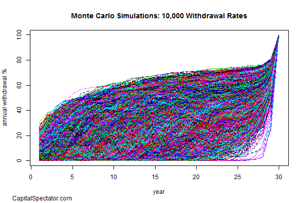
The simulation shows that the withdrawal rates in the first year vary from just a few ticks over zero up to roughly 30%, with a median of roughly 6.1% and an interquartile range of around 2.5% to 10.8%.

This is far from the last word on modeling the possibilities, but it provides a starting outline for further work. If I was running a genuine modeling project, there would be several other facets of analytics to implement. For example, we would take a deeper look at return and risk assumptions for modeling a risky portfolio. As one alternative, we might use actual returns from several real-world portfolios and resample the historical track record. Another possibility is creating synthetic risk and return samples based on various distributions to account for fat tails. In addition, a robust modeling effort should consider investment horizons beyond a finite 30-year period and factor in a range of regime states, such as another financial crisis a la 2008.

In the end, there’s always going to be some level of uncertainty when it comes to projecting “safe” withdrawal rates based on a portfolio of risky assets. The good news is that we can reduce the uncertainty a bit—perhaps substantially—with some informed modeling.

#####

R code to reproduce results/graphs above

[code language=”r”]
# Replicate Excel’s PMT() function in R:
pmt <- function(rate, nper, pv, fv=0, type=0) {
a <- 1/(1+rate)^nper
b <- (-pv-fv*a)*rate/(1-a)
c <-(b/(1+rate*type))
d <-c*0.01
}

# Compute "riskless" withdrawal rates
# based on current 30-year TIPS yield of 1.07% (as of 6/19/2015)
# for a 30-year horizon for a portfolio. The portfolio amount used
# here is 100 in order to compute percentages.
# Note: the final "1" indicates that payments are made
# at the start of each period; a "0" would indicate
# payments at the end of each period
riskless.wr <-pmt(0.0107,30:1,100,,1)*-100

# simulate 100000 withdrawal rates for a risky portfolio
# for a 30-year horizon based on the following assumptions:
# expected real mean return of 4.77%
# expected return volatilty of 10%

set.seed(55) # fixing seed for reproducible random numbers
risky.wr.sim <-replicate(10000,pmt(cumsum(rnorm(n=30, mean=0.0477, sd=0.10)),30:1,100,,1))*-100

# Calculate risk of first-year withdrawal rate sims
range(risky.wr.sim[1,])

# Calculate risk of first-year withdrawal rate sims
quantile(risky.wr.sim[1,])

### create graphs

# Riskless withdrawal rate
plot(riskless.wr,type="h",lwd=3,col="red",
main="Projected Withdrawal Rate",
ylab="annual withdrawal %",
xlab="year")
mtext(side=1,"CapitalSpectator.com",line=-10,adj=0.05,padj=12.7,outer=TRUE)

# Simulated withdrawal rates
matplot(risky.wr.sim,type="l",
main="Monte Carlo Simulations: 10,000 Withdrawal Rates",
ylab="annual withdrawal %",
xlab="year",
ylim=c(0,100))
mtext(side=1,"CapitalSpectator.com",line=-10,adj=0.05,padj=12.7,outer=TRUE)

[/code]