The financial crisis of 2008 devastated portfolios far and wide and brought the global economy to the brink of collapse. It was a disaster, but there was at least one positive outcome from the debacle: a wider recognition that tail risk is a real and present danger that’s forever lurking. The challenge is deciding how to model and manage the risk. You won’t find any easy solutions, but there are practical tools for estimating a portfolio’s vulnerability.

In Part I of tail risk analysis I reviewed the pros and cons of value at risk (VaR) and estimated shortfall (ES), two of the more popular quantitative tools for getting a handle on the probability that an asset or portfolio will suffer an usually steep loss at some point. The limits of these metrics are widely known, particularly for VaR. Can we do better? Yes, according to advocates of extreme value theory (EVT), which is considered a more reliable and robust methodology for estimating the demons that lie in wait in the outliers of the return distributions for assets, markets, and investment portfolios.

EVT traces its theoretical roots to research in the 1920s, but the application for investing is a relatively recent development that begins in the 1990s. The logic for using EVT is that it offers a superior framework for modeling financial market risks – extreme losses in particular.

The main challenge with analyzing so-called left-tail events is the paucity of data. By definition, unusually steep losses that occur, say, 1% of the time are rare, which means that the empirical cupboard is nearly bare. In turn, modeling events that are infrequent is statistically and econometrically challenging, and so the standard metrics are typically useless. EVT attempts to step into the breach with a solution.

As an example, let’s analyze a simple 60/40 stock/bond portfolio, based on the Vanguard 500 Index (VFINX) to represent equities and Vanguard Intermediate-Term Treasury (VFITX) for bonds. The portfolio will be rebalanced back to the target weights at the end of each calendar year, using a start date of Dec. 31, 1991 through yesterday (Feb. 6, 2017). The analytics will be run in R, using the fExtremes package to fit the EVT model. Here’s the code to replicate the results that follow.

Let’s begin with reviewing the full distribution of daily returns for the 60/40 portfolio. As Figure 1 shows, the empirical history can be approximated with a normal distribution (red line), but it’s hardly a perfect fit.

Figure 1

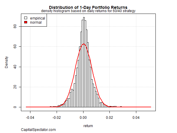
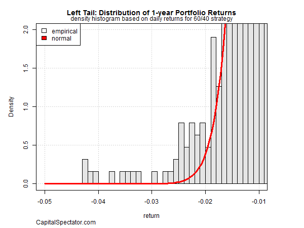
Although Figure 1 appears to show that the losses are normally distributed, reality is quite different once we zoom in on the left side of the tail (i.e., the distribution of the negative returns). In Figure 2, it’s clear that losses occur with greater frequency than a normal distribution allows.

Figure 2

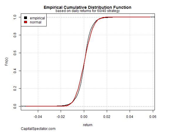
The cumulative distribution function (CDF) provides a more useful tool for visually inspecting the return distribution vs. the standard histogram. The CDF of the 60/40 portfolio returns shows the range of probabilities that a return will be equal to or less than a specific value. For example, the normal distribution line (indicated in red) in Figure 3, as it moves from left to right, reflects a rising probability (vertical axis) of a higher return (horizontal axis). For instance, there’s a roughly 40% probability of a zero-percent (or less) return for the portfolio on any given day. But the empirical history (black line) doesn’t exactly match the red line and so caution is recommended for assuming that a normal distribution applies.

Figure 3

Zooming in on the left-tail portion of the CDF plot (Figure 4) clearly shows that the 60/40 losses occur more frequently than expected via a normal distribution. Yes, the probability of a loss is quite low, according to the empirical record. But that offers little comfort since we know that at some point the 60/40 portfolio will suffer a steep loss, perhaps more frequently and deeply than the historical record implies.

Figure 4

Figure 4 above tells us that the steepest daily loss for the 60/40 portfolio was a bit more than 4%. A naïve review of history would simply accept this decline as the worst-case scenario. Further, the empirical record shows that there were only nine days with losses of 3% or higher – representing a mere 0.14% of the daily returns since 1991. But that low-risk estimate may be an artifact of a specific historical sample. In other words, the historical period we’re using to estimate tail risk may be misleading. How can we develop a higher-confidence estimate of the worst-case scenarios with so little data to analyze? This is where EVT can help. As Jon Danielsson notes in Financial Risk Forecasting ,  “an appealing aspect of EVT is that it does not require a prior assumption about the return distribution….”

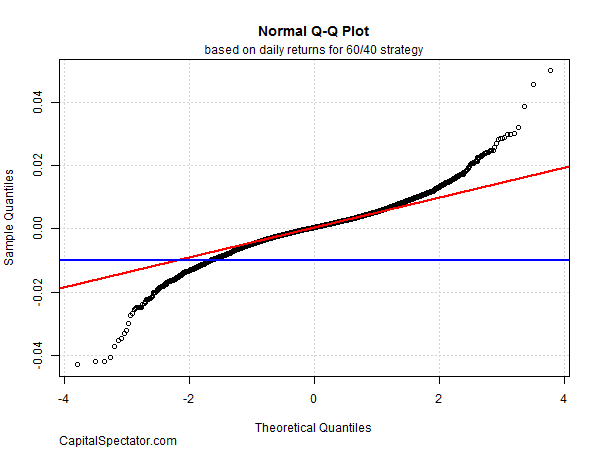
The tricky part of EVT is deciding how to select a threshold value for the returns. There are several methodologies, but for illustration purposes let’s use a simple one by eyeballing the point that appears to separate the left tail from the rest of the distribution. Figure 5 shows a so-called Q-Q plot, which compares the sample quantiles of return with the theoretical quantiles. If the actual returns (black circles) were distributed normally (red line), the circles would align with the red line. That’s true for the center of the distribution, but at the tail ends the circles show significant deviation. The question for EVT modeling is where that deviation begins? As a rough approximation, let’s assume that returns at negative 1% and below define the left tail, as indicated by the horizontal blue line.

Figure 5

Now that we have a 1% threshold estimate we can model the 60/40 portfolio with EVT. One possibility for running the analytics is using a generalized Pareto distribution (GPD), which is a common choice for modeling tail events. As Figure 6 shows, after crunching the numbers it’s clear that the GPD fit (green line) is considerably better for modeling extreme returns vs. the normal distribution (red line).

Figure 6

One way to put the EVT results to work is to estimate VaR and ES with the model parameters. In this case, however, the 60/40 risk estimates via EVT aren’t all that different than the results generated with the conventional techniques for calculating VaR and ES (see Table A). But this may be a function of the 60/40 portfolio. For other investment strategies, the EVT-based estimates of VaR and ES may be considerably different.

Table A

A more powerful application of EVT modeling is running a Monte Carlo simulation to test outcomes that could occur by synthetically creating the equivalent of far longer periods of performance history. In the historical sample above, the data is limited to the 1991-2017 period, which translates to a bit more than 12,600 daily returns. Let’s increase the performance loss sample dramatically by simulating 1 million daily returns based on our EVT modeling above for a deeper read on the left-tail possibilities with the 60/40 portfolio. The result is shown in Figure 7.

Figure 7

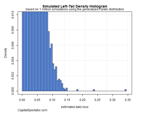
Although the chart appears to profile the right tail, it’s actually showing the left-tail estimates. As you can see, the potential for losses are considerably greater compared with what the 1991-2017 historical record implies. The deepest daily loss in that history was a bit more than 4%. By contrast, the EVT-based simulation above tells us that the losses approaching 35% are possible. As a practical matter, most of the simulated losses max out at roughly 15%. The probability is extremely low of seeing anything larger.

The main point is that an EVT-based evaluation of tail risk for the 60/40 portfolio is substantially higher than history suggests. That doesn’t mean that much bigger losses will occur. But in the interest of stress testing a portfolio it’s crucial to develop a quantitatively reliable estimate of the worst-case scenarios. EVT isn’t perfect, but it may be the best solution compared with the alternatives in the dark art/science of modeling tail risk.