A couple of weeks back I published the first part of a full-chapter excerpt from my new book, Quantitative Investment Portfolio Analytics In R: An Introduction To R For Modeling Portfolio Risk and Return. Here’s the second half of this two-part excerpt of Chapter 5, which reviews the basics for factor analysis via R code. The chapter sample below focuses on additional analytics, including a primer on a close cousin to factor analysis: principal component analysis (PCA).  (Note: for a cleaner read, the footnotes that appear in the book have been removed for this web-based version of the chapter. For a complete list of the book’s chapters, see here. Keep in mind that all the code published in Quantitative Investment Portfolio Analytics In R can be accessed via a single file by way of a link that’s published in the book.)

Chapter 5 (part II)
Factor Analysis

5.2 Exploratory Factor Analysis

The factanal command offers another option for analyzing risk factors. For example, imagine a fund-of-hedge-funds portfolio with six components, each representing a particular risk factor. One question that may come up: What is the least number of factors required to adequately model the portfolio’s volatility? Using the hedge fund returns in the PerformanceAnalytics library, let’s assume that one factor will suffice. Running factanal on the returns confirms that a single factor can be used to effectively model the portfolio. Note that this analysis is based on a relatively high p-value of 0.275, which in this case is an indication that the null hypothesis can’t be rejected. In other words, the analysis shows that there’s no statistically relevant difference between using one factor to model volatility and using the entire portfolio as presented.

[code language=”r”]
library(PerformanceAnalytics)
data(managers)
ret <-na.omit(managers[,1:6])
fit <-factanal(ret, factors=1)
fit

Call:
factanal(x = ret, factors = 1)

Uniquenesses:
HAM1 HAM2 HAM3 HAM4 HAM5 HAM6
0.192 0.771 0.446 0.437 0.726 0.566

Loadings:
Factor1
HAM1 0.899
HAM2 0.478
HAM3 0.745
HAM4 0.750
HAM5 0.524
HAM6 0.659

Factor1
SS loadings 2.862
Proportion Var 0.477

Test of the hypothesis that 1 factor is sufficient.
The chi square statistic is 11.01 on 9 degrees of freedom.
The p-value is 0.275
[/code]

We can visually inspect the one-factor modeling recommendation with prcomp, which performs a principal component analysis (PCA), a methodology for reducing the dimensionality of a dataset (in this case portfolio returns) to identify the key drivers (i.e., the principal components) of the returns. Figure 5.2 graphs the sorted eigenvalues (variances) of the principal components (factors) in descending order. Visual inspection suggests that the first two or three factors are the key sources of portfolio volatility, which implies that the remaining factors can be ignored.

[code language=”r”]
plot(prcomp(ret))
[/code]

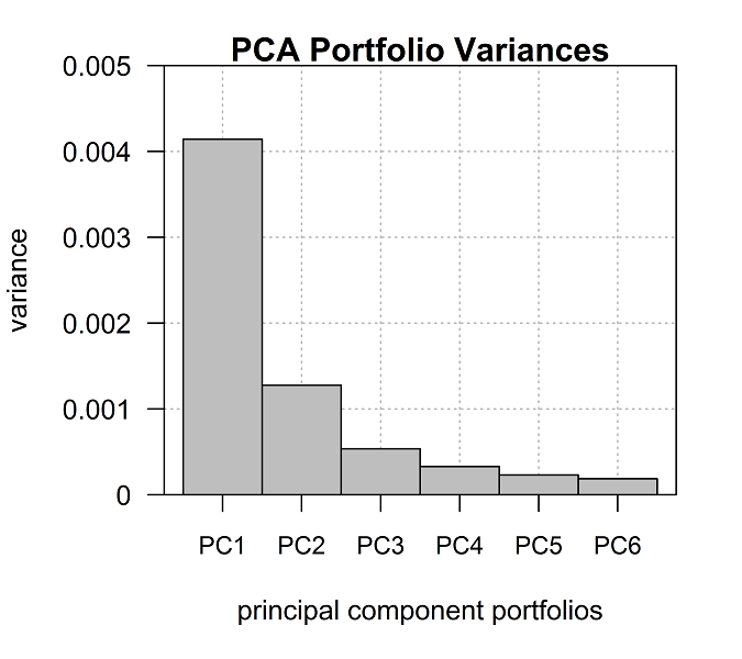
Figure 5.2: PCA portfolio variances

Figure 5.2 clearly shows that the first factor (PC1, or principal component one) is the dominant source of the portfolio’s performance volatility. PC1 is usually a proxy for the “market” beta.7 Factors 2 through 6, by comparison, exhibit decreasing degrees of influence. The additional factors are unnamed and identifying them precisely can be challenging. Statistically speaking, however, the additional factors are easily modeled. Note, too, that all the principal component portfolios, by definition, are orthogonal, which is to say independent (uncorrelated) with each other.

To inspect the PCA data, you can save the output from prcomp and print the results. The output reveals that PC1 represents nearly 62% of the portfolio’s variance.

[code language=”r”]
ret.pc <-prcomp(ret)
print(summary(ret.pc),digits=3)

Importance of components:
PC1 PC2 PC3 PC4 PC5 PC6
Standard deviation 0.0644 0.0357 0.0232 0.0182 0.0152 0.0137
Proportion of Variance 0.6179 0.1905 0.0800 0.0491 0.0345 0.0280
Cumulative Proportion 0.6179 0.8084 0.8884 0.9375 0.9720 1.0000
[/code]

One possible use of the data is replicating one or more of the factor portfolios. For example, to replicate the first factor portfolio using the six hedge funds we can extract the weights from the PCA data by calculating eigenvectors for each factor via the eigenvalues. The resulting portfolios are known as eigenportfolios, with the asset weights for each captured in wgt.1.

[code language=”r”]
wgt.1 <-apply(ret.pc$rotation,2,function(x) x/sum(x))
round(wgt.1,4)
PC1 PC2 PC3 PC4 PC5 PC6
HAM1 0.1739 0.1389 0.2258 -2.7164 -0.7850 19.1821
HAM2 0.0654 0.1337 0.4749 2.6263 5.2086 4.4072
HAM3 0.1201 0.1597 0.5063 -3.1222 0.7844 -15.4557
HAM4 0.3669 -0.6759 -0.3700 0.6202 0.7804 -3.3440
HAM5 0.1576 1.2420 -0.3434 0.7566 -0.1432 -2.4513
HAM6 0.1160 0.0015 0.5065 2.8355 -4.8451 -1.3383
[/code]

The eigenportfolios are unnamed, but replicating one or more is straightforward.
For example, the first factor portfolio (PC1), the “market” portfolio, can be
constructed from the eigenvectors (weights), which sum to 1.0.

[code language=”r”]
sum(wgt.1[,1])
[1] 1
[/code]

The remaining portfolios target other factors, which are unidentified. Depending on the portfolio under review, the additional factor portfolios may target any number of financial and/or macro factors, such as inflation, economic growth, interest rates, etc. The caveat is that the lower the eigenvalue (variance linked to the variables) for a given eigenportfolio, the lower the explanatory power. The sixth portfolio (PC6) in the example above, for instance, has almost no explanatory power and so this portfolio’s value as an investment that resonates will likely be nil.

As another example of PCA modeling, let’s review a portfolio comprised of five ETFs. For the historical fund prices, we’ll tap into Yahoo Finance’s free database via getSymbols in the quantmod package.

[code language=”r”]
library(quantmod)
symbols <-c("SPY", "AGG", "EFA", "EEM", "OIL")
getSymbols(symbols, src = "yahoo", auto.assign=T)
prices <- do.call(merge, lapply(symbols, function(x) Cl(get(x))))
colnames(prices) <-symbols
[/code]

To create the prices file above, lapply extracts the column of downloaded closing prices for each time series via the Cl(get(x)) commands. The get command searches for an object by name, in this case each of the symbols listed in symbols. Because get is wrapped in Cl, which extracts closing prices, the get search targets only closing prices. Note, too, that Cl(get(x)) is executed as a function in lapply. The resulting output – five columns of closing prices as per symbols – is combined in the prices file using merge via do.call, which calls and executes all the commands. Finally, each column is labeled with the appropriate symbol by way of colnames.

The output files for lapply are formatted as lists, which is one of several types of objects available in R. In this task, working with lists makes the necessary cutting and pasting easier. As a result, lapply is useful here because we need to extract the adjusted closing price for each ticker and then combine the results in one file by column.

With the prices file in hand, the next step is generating returns and running the PCA.

[code language=”r”]
ret <-na.omit(ROC(prices[‘2007-12-31::2016-12-31’],
1,
"discrete",
na.pad = FALSE))

fit <-prcomp(ret)
factors.1 <-round(fit$rotation,3)
factors.1

PC1 PC2 PC3 PC4 PC5
SPY 0.360 -0.261 0.465 0.748 -0.162
AGG -0.011 -0.002 0.023 -0.220 -0.975
EFA 0.450 -0.300 0.542 -0.625 0.150
EEM 0.592 -0.399 -0.700 0.005 -0.024
OIL 0.563 0.826 0.006 0.011 -0.010
[/code]

The output shows that the first factor portfolio – PC1, or the “market” portfolio – is heavily influenced by SPY, EFA, and EEM – equity funds. The OIL fund, a crude oil portfolio, also ranks high as a relevant driver of results. By contrast, the lone bond fund – AGG – doesn’t resonate, as indicated by its roughly zero loading.

Turning to the weights, the PC1 “market” portfolio is allocated to the equity and
oil ETFs, with a roughly zero weight in bonds (AGG).

[code language=”r”]
wgt.a <-apply(fit$rotation,2,function(x) x/sum(x))
round(wgt.a[,1],2)
SPY AGG EFA EEM OIL
0.18 -0.01 0.23 0.30 0.29
[/code]