I’ve been analyzing a 60/40 US stock/bond portfolio in R in a series of posts and today’s installment picks up from the previous post by adding a global strategy. The goal is enhancing the 60/40’s return while keeping risk at a comparable if not lesser level. Overly ambitious? Perhaps, but it’s still valuable to explore the historical record.

A thorough analysis will require several posts, and so today’s update will only consider the preliminaries, including a simple performance comparison of how the 60/40 strategy stacks up against a global portfolio with rebalanced and buy-and-hold variations. As a preview, the global strategy delivers a slightly higher return over the sample period (the close of 2003 through Feb. 13, 2014). The results inspire a deeper round of analysis, which is forthcoming. Meantime, today’s data focuses our attention on a curious pattern: the global strategy delivered a solid round of improvement early on, but gave up most/all of the edge in the 2008 market crash. The superior results returned in the post-crash period, but the edge faded in recent months. Hmmm.

I’ll be exploring the implications of this behavior in future posts, with an emphasis on looking for real-world solutions for tweaking the portfolio design and rebalancing rules in order to capture and hold on to the global strategy’s advantages.

Meanwhile, let’s set up the basic template and review some housekeeping details. First, how should we create a global strategy? There are many possibilities, but for now we’ll begin with a relatively simple design. Using the 60/40 stock/bond mix as a foundation, we’ll take five percentage points from each asset and reallocate to so-called alternatives: a broad-basket definition of commodities and real estate (real estate investment trusts). For the remaining stocks and bonds, we’ll divide allocations into a more granulate set of US and foreign allocations as follows:

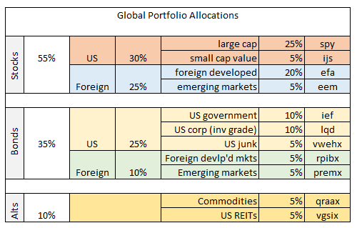
The resulting allocation is moderately subjective. For good or ill, the portfolio mix serves our goal of a simplicity in terms of round numbers that aren’t too extreme. In short, a decent first approximation of weights to run a backtest. Could we do better? Probably, and so this is a subject that’s worth exploring later on.

Keep in mind that we’re now using mutual funds as well as ETFs in order to maintain the same starting date (Dec. 31, 2003) that was used in the 60/40 analysis (note the list of tickers in the far-right-hand column). ETFs have a relatively limited history, particularly when moving beyond US stocks and bonds. The limitation requires looking for alternative open-end products in search of a sufficiently long track records to run a backtest. In some cases there are superior funds available for building a portfolio today. But I’ve made some comprises in the interest of crunching the numbers with a single, continuous set of real-world performance histories for the sample period. As for the R code, you’ll find it below.

Meantime, let’s cut to the chase and review how the strategies compare based on a $1 investment at the close of 2003. The first chart shows that the global portfolio delivered slightly stronger results during the test period via a buy-and-hold strategy. A $1 investment in the 60/40 strategy more than doubled to $2.06 through last Friday’s close (Feb. 13); the global portfolio did a bit better, rising to $2.08.

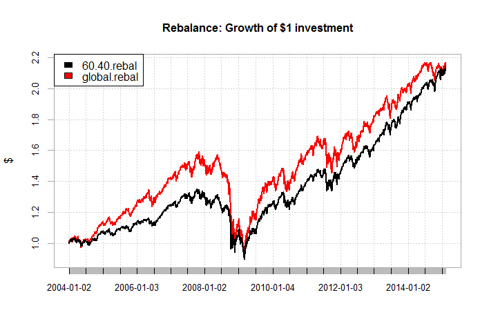
Rebalancing the portfolios every Dec. 31 back to the initial allocations in the table above delivered slightly higher returns, albeit not by much: $2.14 for 60/40 and $2.17 via the global strategy.

It’s interesting to note that the global strategy was delivering substantially stronger results over the 60/40 portfolio at times. Is it possible to modify the strategy to boost the odds of preserving those stronger gains? I’ll focus on these and related questions/analytics the next time. Meanwhile, you can find links of the previous articles in this series at the bottom of this post.

[code language=”r”]

# load packages
library(quantmod)
library(tseries)
library(PerformanceAnalytics)

# download prices
# 60/40 portfolio
spy <-get.hist.quote(instrument="spy",start="2003-12-31",quote="AdjClose",compression="d")
agg <-get.hist.quote(instrument="agg",start="2003-12-31",quote="AdjClose",compression="d")

# global portfolio
spy <-get.hist.quote(instrument="spy",start="2003-12-31",quote="AdjClose",compression="d") # us broad equities
ijs <-get.hist.quote(instrument="ijs",start="2003-12-31",quote="AdjClose",compression="d") # us small cap value equities

efa <-get.hist.quote(instrument="efa",start="2003-12-31",quote="AdjClose",compression="d") # foreign developed equities
eem <-get.hist.quote(instrument="eem",start="2003-12-31",quote="AdjClose",compression="d") # emg mkt equities

ief <-get.hist.quote(instrument="ief",start="2003-12-31",quote="AdjClose",compression="d") # us gov’t bonds
lqd <-get.hist.quote(instrument="lqd",start="2003-12-31",quote="AdjClose",compression="d") # us corp bonds/investment grade
vwehx <-get.hist.quote(instrument="vwehx",start="2003-12-31",quote="AdjClose",compression="d") # us junk bonds

rpibx <-get.hist.quote(instrument="rpibx",start="2003-12-31",quote="AdjClose",compression="d") # for devlp’d bonds
premx <-get.hist.quote(instrument="premx",start="2003-12-31",quote="AdjClose",compression="d") # emg mtk bonds

qraax <-get.hist.quote(instrument="qraax",start="2003-12-31",quote="AdjClose",compression="d") # commodities
vgsix <-get.hist.quote(instrument="vgsix",start="2003-12-31",quote="AdjClose",compression="d") # us reits

# select asset weights
w.60.40 = c(0.6,0.4) # 60% / 40%
w.global = c(0.25,0.05,0.20,0.05,0.10,0.10,0.05,0.05,0.05,0.05,0.05) # global aa

# merge price histories into one dataset
# calculate 1-day % returns and label columns
port.60.40.prices <-as.xts(merge(spy,agg))
port.60.40.returns <-na.omit(ROC(port.60.40.prices,1,"discrete"))
colnames(port.60.40.returns) <-c("spy","agg")

port.global.prices <-as.xts(merge(spy,ijs,efa,eem,ief,lqd,vwehx,rpibx,premx,qraax,vgsix))
port.global.returns <-na.omit(ROC(port.global.prices,1,"discrete"))
colnames(port.global.returns) <-c("spy","ijs","efa","eem","ief","lqd","vwehx","rpibx","premx","qraax","vgsix")

# calculate weighted total returns for portfolios

# buy and hold portfolio/no rebalancing
port.60.40.bh <-Return.portfolio(port.60.40.returns,
weights=w.60.40,wealth.index=TRUE,verbose=TRUE)

port.global.bh <-Return.portfolio(port.global.returns,
weights=w.global,wealth.index=TRUE,verbose=TRUE)
# year-end rebalanced portfolios
port.60.40.rebal <-Return.portfolio(port.60.40.returns,
rebalance_on="years",
weights=w.60.40,wealth.index=TRUE,verbose=TRUE)

port.global.rebal <-Return.portfolio(port.global.returns,
rebalance_on="years",
weights=w.global,wealth.index=TRUE,verbose=TRUE)

# merge portfolio returns into datasets based on strategy
# buy & hold
port.bh <-merge(port.60.40.bh$returns,port.global.bh$returns)
colnames(port.bh) <-c("60.40.bh","global.bh")

# rebalance
port.rebal <-merge(port.60.40.rebal$returns,port.global.rebal$returns)
colnames(port.rebal) <-c("60.40.rebal","global.rebal")

# create strategy performance charts
chart.CumReturns(port.bh,
wealth.index=TRUE,
main="Buy & Hold: Growth of $1 investment",
ylab="$")
legend("topleft",c(colnames(port.bh)),cex=1,fill=(c("black","red")))

chart.CumReturns(port.rebal,
wealth.index=TRUE,
main="Rebalance: Growth of $1 investment",
ylab="$")
legend("topleft",c(colnames(port.rebal)),cex=1,fill=(c("black","red")))
[/code]

Portfolio Analysis in R: Part I | A 60/40 US Stock/Bond Portfolio
Portfolio Analysis in R: Part II | Analyzing A 60/40 Strategy