The expected risk premium for the Global Market Index (GMI) fell to an annualized 4.2% in December, moderately below the 4.6% estimate in the previous month. The revised projection for GMI (an unmanaged market-value-weighted portfolio that holds all the major asset classes) represents the ex ante premium over the projected “risk-free” rate for the long run.

Adjusting for short-term momentum and medium-term mean-reversion factors (defined below) generates a fractionally higher ex ante risk premium for GMI: an annualized 4.3% forecast.

The projections remain well below GMI’s historical performance for the trailing 10-year period through last month. The benchmark earned a solid 6.7% annualized risk premium for the decade through December 2018, substantially above GMI’s current unadjusted 4.2% long-run forecast.

All forecasts are likely to be wrong to some degree, but the projections for GMI are expected to be somewhat more reliable vs. the estimates for the individual asset classes. Predictions for the market components are subject to greater uncertainty compared with aggregating forecasts, a process that may cancel out some of the errors through time.

Learn To Use R For Portfolio Analysis
Quantitative Investment Portfolio Analytics In R:
An Introduction To R For Modeling Portfolio Risk and Return
By James Picerno

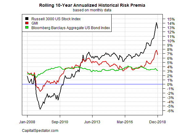
For a bit of historical perspective, consider the chart below, which shows the rolling 10-year annualized risk premia for GMI, US stocks (Russell 3000), and US Bonds (Bloomberg Aggregate Bond) through last month. Note that GMI’s current 10-year performance (red line) has pulled back recently, but remains elevated compared with results over the past decade.

Now let’s turn to a summary of the methodology and rationale for the estimates above. The basic idea is to reverse engineer expected return, based on risk assumptions. Rather than trying to predict return directly, this approach relies on the moderately more reliable model of using risk metrics to estimate the performances of asset classes. The process is relatively robust in the sense that forecasting risk is slightly easier than projecting return. With the necessary data in hand, we can calculate the implied risk premia with the following inputs:

● an estimate of GMI’s expected market price of risk, defined as the Sharpe ratio, which is the ratio of risk premia to volatility (standard deviation).
● the expected volatility (standard deviation) of each asset
● the expected correlation for each asset with the overall portfolio (GMI)

The estimates are drawn from the historical record since the close of 1997 and are presented as a first approximation for modeling the future. The projected premium for each asset class is calculated as the product of the three inputs above. GMI’s ex ante risk premia is computed as the market-value-weighted sum of the individual projections for the asset classes.

The framework for estimating equilibrium returns was initially outlined in a 1974 paper by Professor Bill Sharpe. For a more practical-minded summary, see Gary Brinson’s explanation of the process in Chap. 3 of The Portable MBA in Investment. I also review the model in my book Dynamic Asset Allocation. Here’s how Robert Litterman explains the concept of equilibrium risk premium estimates in Modern Investment Management: An Equilibrium Approach:

We need not assume that markets are always in equilibrium to find an equilibrium approach useful. Rather, we view the world as a complex, highly random system in which there is a constant barrage of new data and shocks to existing valuations that as often as not knock the system away from equilibrium. However, although we anticipate that these shocks constantly create deviations from equilibrium in financial markets, and we recognize that frictions prevent those deviations from disappearing immediately, we also assume that these deviations represent opportunities. Wise investors attempting to take advantage of these opportunities take actions that create the forces which continuously push the system back toward equilibrium. Thus, we view the financial markets as having a center of gravity that is defined by the equilibrium between supply and demand. Understanding the nature of that equilibrium helps us to understand financial markets as they constantly are shocked around and then pushed back toward that equilibrium.

The adjusted risk premia estimates in the table above reflect changes based on two factors: short-term momentum and long-term mean reversion. Momentum is defined here as the current price relative to the trailing 10-month moving average. The mean reversion factor is estimated as the current price relative to the trailing 36-month moving average. The raw risk premia estimates are adjusted based on current prices relative to the 10-month and 36-month moving averages. If current prices are above (below) the moving averages, the unadjusted risk premia estimates are decreased (increased). The formula for adjustment is simply taking the inverse of the average of the current price to the two moving averages as the signal for modifying the projections. For example: if an asset class’s current price is 10% above it’s 10-month moving average and 20% over its 36-month moving average, the unadjusted risk premium estimate is reduced by 15% (the average of 10% and 20%).

What can you do with the forecasts in the table above? You might start by considering if the expected risk premia are satisfactory… or not. If the estimates fall short of your required return, you might consider how to engineer a higher rate of performance by way of customizing asset allocation and rebalancing rules. Keep in mind that GMI’s raw implied risk premia are based on an unmanaged market-value weighted mix of the major asset classes. In theory, that’s the optimal asset allocation for the average investor with an infinite time horizon. Unless you’re a foundation or pension fund, this time-horizon assumption is impractical and so there’s a reasonable case for a) modifying Mr. Market’s asset allocation to suit your particular needs and risk budget; and b) adding a rebalancing component to your investment strategy.

You might also estimate risk premia with alternative methodologies for additional insight about the near-term future (an excellent resource on this subject: Antti Ilmanen’s Expected Returns). For instance, let’s say that you have confidence in the dividend-discount model (DDM) for predicting equity market performance over the next 3 to 5 years. After crunching the numbers, you find that DDM tells you that the stock market’s expected performance will differ by a considerable degree vs. the equilibrium-based estimate for the long run. In that case, you have some tactical information to consider.

Keep in mind, too, that combining forecasts via several models may provide a more reliable set of predictions vs. estimates from any one model. Indeed, a number of studies published through the years document that combined forecasts tend to be more robust vs. single-model projections.

What you can’t do is get blood out of a stone. No one really knows what risk premia will be in the months and years ahead, which is why relying on forecasting alone (particularly for the short-term future) is asking for trouble. In other words, you should deviate from Mr. Market’s asset allocation carefully, thoughtfully, and for reasons other than assuming that you’re smarter than everyone else (i.e., the market).