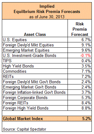
If you built a portfolio with a market-value weighted mix of all the major asset classes, what risk premium would you expect? I’m looking for a 5.2% return, give or take. To be more precise, my current equilibrium-based forecast of total return (less the risk-free rate) for the Global Market Index (GMI) is 5.2% these days.
Yes, that’s a forecast, and so it comes with all the usual caveats, but it’s a prediction that I’m inclined to use as a base-case scenario for looking ahead (as of mid-year 2013). Why? Several reasons, including the recognition that analyzing the future by this roadmap, for a multi-asset class portfolio, tends to offer a reasonable guesstimate. When you look for implied returns via computing risk estimates, and do so for a broad set of asset classes, the inevitable errors tend to be less severe compared with trying to predict return directly for, say, stocks alone.
For those who aren’t familiar with equilibrium estimates of expected return, the short explanation of the process is that the predictions are an estimate of what you’d earn through time on the assumption that markets clear. An heroic assumption? Probably, but still useful, particularly if we run the numbers periodically and look for trends. By that standard, nothing much has changed. My equilibrium estimate for GMI is still in the ~5.0% range, as it has been all year.
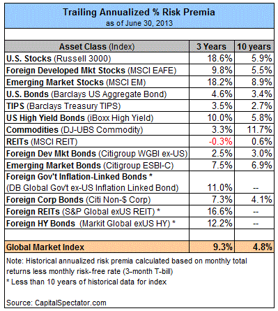
Before I dive into how I came up with that forecast, let’s consider where we’ve been. Here’s how risk premia for the major asset classes stacks up in recent history. Remember, we’re looking at risk premia, or total return less the risk-free rate, which I’m defining by way of the three-month T-bill return.

Next, here’s how the major asset classes compare in terms of the Sharpe ratio, a popular risk metric that’s based on the ratio of a risk premium to its volatility. Higher (lower) Sharpe ratios equate with higher (lower) returns per unit of risk. There are alternative risk metrics to consider, but for simplicity (and tradition) here I’ll stick with the Sharpe ratio.

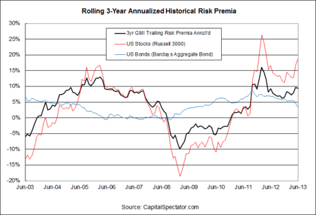
For additional context, here’s how GMI’s rolling three-year annualized risk premium (black line) looks next to the equivalent for US stocks (Russell 3000) and US bonds (Barclays Aggregate). As you can see, historical risk premia are an unstable species, and we should expect no less when looking ahead. Today’s estimate, in other words, won’t be relevant tomorrow.

Speaking of forward-looking estimates, here’s the big-picture, including GMI’s equilibrium risk premium prediction:

What’s the recipe for the forecasts above? The short answer is that I’m using assumptions for three inputs: an estimate of the market’s price of risk (Sharpe ratio), return volatility for the asset classes and GMI, and correlations between those assets and the portfolio (GMI). In this case, I’m not using a terribly sophisticated modeling system for the estimates. Instead, I’m taking the trailing 10-year Sharpe ratio for GMI as the proxy for the market’s price of risk. For the volatility and correlation numbers, the trailing three-year numbers are used.
Where does the idea for using an equilibrium-based forecast come from? I’m using a slightly adjusted framework originally laid out by Professor Bill Sharpe in a 1974 paper in the Journal of Financial and Quantitative Analysis: “Imputing Expected Returns From Portfolio Composition.” For a slightly less-geeky overview, see the “Reverse Optimization” section in Thomas Idzorek’s monograph or Chapter 3 by Gary Brinson in The Portable MBA in Investment. I also discuss the basic process in Chapter 9 of my book Dynamic Asset Allocation: Modern Portfolio Theory Updated for the Smart Investor
.
What’s the practical value here? Not much, if you’re expecting that any one set of estimates tells you most of what you need to know. Rather, I prefer to look at equilibrium estimates periodically and compare how (or if) they change. If the numbers are routinely trending down, or up, that tells you something. The fact that the ~5.0% projection has more or less remained steady lately is also valuable information.
Keep in mind that the realized risk premia for GMI has fluctuated around the 5% mark in recent history. It’s best to assume no less for the near term. For the moment, the fluctuations have been on the high side of 5%, but one day we’ll see the flip side of that happy state of affairs. But that’s a tactical topic for another day. The goal of an equilibrium-based outlook, by contrast, is one of considering what the markets will dispense, in the aggregate, over a longer time horizon. The outcome for next month (or even next year) is something else entirely.
Yes, it’s all an academic exercise to some extent. But the inevitable flaws are probably muted when we aggregate the individual forecasts up into GMI’s projection. Even if you’re inclined to disagree with the assumptions above, the framework is still useful because of its flexibility. You could, for instance, apply a different (superior?) methodology for the volatility estimates vs. using recent history. You might also stress test the equilibrium forecast by projecting risk premia with other applications, such as forecasting equity returns via dividend yields or earnings estimates.
The sky’s the limit for guessing what Mr. Market’s asset allocation will dispatch in the years to come. Why should we assume that an equilibrium model deserves a spot on the short list? One reason is that its underlying principles—the markets clear over time—implies that it’s tough to beat GMI (or a comparable proxy) on a sustained basis. Actually, that’s the general message in the empirical record, or at least it has been in recent history.
In that case, developing some intuition about Mr. Market’s asset allocation is a worthy if limited goal. It’s no crystal ball, but it’s a reasonable way to begin, which is more than you can say for most efforts that some folks try to pass off as the basis for a prudent strategy session.